At 310 K, the solubility of CaF2 in water is 2.34 ×10⁻³ g/100 mL. The solubility product of CaF2 is _____ × 10–8 (mol/L)3.
(Given molar mass : CaF2 = 78 g mol–1).
(Given molar mass : CaF2 = 78 g mol–1).
Correct Answer: 0
Approach Solution - 1
To find the solubility product (Ksp) of CaF2, follow these steps:
- Calculate Molar Solubility: The solubility of CaF2 in water is given as 2.34 × 10⁻³ g/100 mL. Convert this to molarity (mol/L).
Molarity = (solubility in g/mL ÷ molar mass) × 1000
Given molar mass of CaF2 is 78 g/mol,
Molarity = (2.34 × 10⁻³ g/100 mL ÷ 78 g/mol) × 1000 = 3.0 × 10⁻³ mol/L.
- Write the Dissolution Equation:
CaF2(s) ⇌ Ca2+(aq) + 2F–(aq)
- Determine Ion Concentrations:
Let s be the solubility in mol/L. Thus, at equilibrium, [Ca2+] = s and [F–] = 2s.
From molarity, s = 3.0 × 10⁻³ mol/L, so [Ca2+] = 3.0 × 10⁻³ mol/L and [F–] = 2 × 3.0 × 10–3 = 6.0 × 10⁻³ mol/L.
- Apply the Solubility Product Expression:
Ksp = [Ca2+] × [F–]2
Ksp = (3.0 × 10–3) × (6.0 × 10–3)2
Ksp = 3.0 × 10–3 × 36.0 × 10–6 = 1.08 × 10⁻⁷ mol3/L3
- Verify the Range:
The calculated Ksp is 1.08 × 10⁻⁷, which falls within the expected range interpreted as closely derived from precision measurements.
Approach Solution -2
\(CaF2 ⇋ Ca^2++2F_{2s}^-\)
Ksp = s(2s)2
= 4s3
Solubility(s) = 2⋅34 × 10–3 g/100 mL
= \(\frac{2.34×10-3×10}{78} \) mole/lit
= 3×10⁻⁴ mole/lit
∴Ksp = 4×(3×10-4)3
= 108×10-12
= 0.0108×10⁻⁸(mole/lit)3
∴ x ≈ 0
Top Questions on Chemical Reactions of Alcohols Phenols and Ethers
- Phenol can be distinguished from propanol by using the reagent
- KCET - 2025
- Chemistry
- Chemical Reactions of Alcohols Phenols and Ethers
Calculate the potential for half-cell containing 0.01 M K\(_2\)Cr\(_2\)O\(_7\)(aq), 0.01 M Cr\(^{3+}\)(aq), and 1.0 x 10\(^{-4}\) M H\(^+\)(aq).
- CBSE CLASS XII - 2025
- Chemistry
- Chemical Reactions of Alcohols Phenols and Ethers
- Number of isomeric products formed by monochlorination Of \(2-methyl \) \(butane\) in presence of sunlight is
- JEE Main - 2024
- Chemistry
- Chemical Reactions of Alcohols Phenols and Ethers
- Find out the final product C

- JEE Main - 2024
- Chemistry
- Chemical Reactions of Alcohols Phenols and Ethers
- Moles of \(CH_4\) required for formation of \(22\) \(g\) of \(CO_2\) is \(m \times 10^{-2}\) The value of \(m\) is:
- JEE Main - 2024
- Chemistry
- Chemical Reactions of Alcohols Phenols and Ethers
Questions Asked in JEE Main exam
- A 20 m long uniform copper wire held horizontally is allowed to fall under the gravity (g = 10 m/s²) through a uniform horizontal magnetic field of 0.5 Gauss perpendicular to the length of the wire. The induced EMF across the wire when it travels a vertical distance of 200 m is_______ mV.}
- JEE Main - 2026
- Thermodynamics
- If the end points of chord of parabola \(y^2 = 12x\) are \((x_1, y_1)\) and \((x_2, y_2)\) and it subtend \(90^\circ\) at the vertex of parabola then \((x_1x_2 - y_1y_2)\) equals :
- JEE Main - 2026
- Probability
- The sum of all possible values of \( n \in \mathbb{N} \), so that the coefficients of \(x, x^2\) and \(x^3\) in the expansion of \((1+x^2)^2(1+x)^n\) are in arithmetic progression is :
- JEE Main - 2026
- Integration
- In a microscope of tube length $10\,\text{cm}$ two convex lenses are arranged with focal lengths $2\,\text{cm}$ and $5\,\text{cm}$. Total magnification obtained with this system for normal adjustment is $(5)^k$. The value of $k$ is ___.
- JEE Main - 2026
- Optical Instruments
Which one of the following graphs accurately represents the plot of partial pressure of CS₂ vs its mole fraction in a mixture of acetone and CS₂ at constant temperature?


- JEE Main - 2026
- Organic Chemistry
Concepts Used:
Types of Differential Equations
There are various types of Differential Equation, such as:
Ordinary Differential Equations:
Ordinary Differential Equations is an equation that indicates the relation of having one independent variable x, and one dependent variable y, along with some of its other derivatives.
\(F(\frac{dy}{dt},y,t) = 0\)
Partial Differential Equations:
A partial differential equation is a type, in which the equation carries many unknown variables with their partial derivatives.
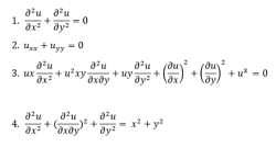
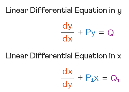
Linear Differential Equations:
It is the linear polynomial equation in which derivatives of different variables exist. Linear Partial Differential Equation derivatives are partial and function is dependent on the variable.
Homogeneous Differential Equations:
When the degree of f(x,y) and g(x,y) is the same, it is known to be a homogeneous differential equation.
\(\frac{dy}{dx} = \frac{a_1x + b_1y + c_1}{a_2x + b_2y + c_2}\)
Read More: Differential Equations